
electromagnetism relating to the operating principles of transformers, inductors, and many types of electrical motors and generators.[1] The law states that:

 Faraday's diskIn Faraday's first experimental demonstration of electromagnetic induction (August 1831), he wrapped two wires around opposite sides of an iron torus (an arrangement similar to a modern transformer). Based on his assessment of recently-discovered properties of electromagnets, he expected that when current started to flow in one wire, a sort of wave would travel through the ring and cause some electrical effect on the opposite side. He plugged one wire into a galvanometer, and watched it as he connected the other wire to a battery. Indeed, he saw a transient current (which he called a "wave of electricity") when he connected the wire to the battery, and another when he disconnected it.[4] Within two months, Faraday had found several other manifestations of electromagnetic induction. For example, he saw transient currents when he quickly slid a bar magnet in and out of a coil of wires, and he generated a steady (DC) current by rotating a copper disk near a bar magnet with a sliding electrical lead ("Faraday's disk").[5]
Faraday explained electromagnetic induction using a concept he called lines of force. However, scientists at the time widely rejected his theoretical ideas, mainly because they were not formulated mathematically.[6] An exception was Maxwell, who used Faraday's ideas as the basis of his quantitative electromagnetic theory.[6][7][8] In Maxwell's papers, the time varying aspect of electromagnetic induction is expressed as a differential equation which Oliver Heaviside referred to as Faraday's law even though it is slightly different in form from the original version of Faraday's law, and doesn't cater for motionally induced EMF. Heaviside's version is the form recognized today in the group of equations known as Maxwell's equations.
Lenz's law, formulated by Heinrich Lenz in 1834, describes "flux through the circuit", and gives the direction of the induced electromotive force and current resulting from electromagnetic induction (elaborated upon in the examples below).
 Faraday's experiment showing induction between coils of wire: The liquid battery (right) provides a current which flows through the small coil (A), creating a magnetic field. When the coils are stationary, no current is induced. But when the small coil is moved in or out of the large coil (B), the magnetic flux through the large coil changes, inducing a current which is detected by the galvanometer (G).[9]
 The definition of surface integral relies on splitting the surface Σ into small surface elements. Each element is associated with a vector dA of magnitude equal to the area of the element and with direction normal to the element and pointing outward.
  A vector field F(r, t) defined throughout space, and a surface Σ bounded by curve ∂Σ moving with velocity v over which the field is integrated.Faraday's law of induction makes use of the magnetic flux ΦB through a surface Σ, defined by an integral over a surface:
 done (per unit charge) moving a test charge around the closed curve ∂Σ(t), called the electromotive force (EMF), is given by:
 is the magnitude of the electromotive force (EMF) in volts and ΦB is the magnetic flux in webers. The direction of the electromotive force is given by Lenz's law.
For a tightly-wound coil of wire, composed of N identical loops, each with the same ΦB, Faraday's law of induction states that
In choosing a path ∂Σ(t) to find EMF, the path must satisfy the basic requirements that (i) it is a closed path, and (ii) the path must capture the relative motion of the parts of the circuit (the origin of the t-dependence in ∂Σ(t) ). It is not a requirement that the path follow a line of current flow, but of course the EMF that is found using the flux law will be the EMF around the chosen path. If a current path is not followed, the EMF might not be the EMF driving the current.
 Figure 3: Closed rectangular wire loop moving along x-axis at velocity v in magnetic field B that varies with position x.Consider the case in Figure 3 of a closed rectangular loop of wire in the xy-plane translated in the x-direction at velocity v. Thus, the center of the loop at xC satisfies v = dxC / dt. The loop has length ℓ in the y-direction and width w in the x-direction. A time-independent but spatially varying magnetic field B(x) points in the z-direction. The magnetic field on the left side is B( xC − w / 2), and on the right side is B( xC + w / 2). The electromotive force is to be found by using either the Lorentz force law or equivalently by using Faraday's induction law above.
The equivalence of these two approaches is general and, depending on the example, one or the other method may prove more practical.
 Figure 4: Rectangular wire loop rotating at angular velocity ω in radially outward pointing magnetic field B of fixed magnitude. Current is collected by brushes attached to top and bottom discs, which have conducting rims.Figure 4 shows a spindle formed of two discs with conducting rims and a conducting loop attached vertically between these rims. The entire assembly spins in a magnetic field that points radially outward, but is the same magnitude regardless of its direction. A radially oriented collecting return loop picks up current from the conducting rims. At the location of the collecting return loop, the radial B-field lies in the plane of the collecting loop, so the collecting loop contributes no flux to the circuit. The electromotive force is to be found directly and by using Faraday's law above.
Consequently, the EMF is
To use the flux rule, we have to look at the entire current path, which includes the path through the rims in the top and bottom discs. We can choose an arbitrary closed path through the rims and the rotating loop, and the flux law will find the EMF around the chosen path. Any path that has a segment attached to the rotating loop captures the relative motion of the parts of the circuit.
As an example path, let's traverse the circuit in the direction of rotation in the top disc, and in the direction opposite to the direction of rotation in the bottom disc (shown by arrows in Figure 4). In this case, for the moving loop at an angle θ from the collecting loop, a portion of the cylinder of area A = r ℓ θ is part of the circuit. This area is perpendicular to the B-field, and so contributes to the flux an amount:
Now let's try a different path. Follow a path traversing the rims via the opposite choice of segments. Then the coupled flux would decrease as θ increased, but the right-hand rule would suggest the current loop added to the applied B-field, so the EMF around this path is the same as for the first path. Any mixture of return paths leads to the same result for EMF, so it is actually immaterial which path is followed.
 Figure 5: A simplified version of Figure 4. The loop slides with velocity v in a stationary, homogeneous B-field.The use of a closed path to find EMF as done above appears to depend upon details of the path geometry. In contrast, the Lorentz-law approach is independent of such restrictions. The following discussion is intended to provide a better understanding of the equivalence of paths and escape the particulars of path selection when using the flux law.
Figure 5 is an idealization of Figure 4 with the cylinder unwrapped onto a plane. The same path-related analysis works, but a simplification is suggested. The time-independent aspects of the circuit cannot affect the time-rate-of-change of flux. For example, at a constant velocity of sliding the loop, the details of current flow through the loop are not time dependent. Instead of concern over details of the closed loop selected to find the EMF, one can focus on the area of B-field swept out by the moving loop. This suggestion amounts to finding the rate at which flux is cut by the circuit.[15] That notion provides direct evaluation of the rate of change of flux, without concern over the time-independent details of various path choices around the circuit. Just as with the Lorentz law approach, it is clear that any two paths attached to the sliding loop, but differing in how they cross the loop, produce the same rate-of-change of flux.
In Figure 5 the area swept out in unit time is simply dA / dt = v ℓ, regardless of the details of the selected closed path, so Faraday's law of induction provides the EMF as:[16]
 Figure 6: An illustration of Kelvin-Stokes theorem with surface Σ its boundary ∂Σ and orientation n set by the right-hand rule.A changing magnetic field creates an electric field; this phenomenon is described by the Maxwell-Faraday equation:[17]
It can also be written in an integral form by the Kelvin-Stokes theorem:[18]
The integral around ∂Σ is called a path integral or line integral. The surface integral at the right-hand side of the Maxwell-Faraday equation is the explicit expression for the magnetic flux ΦB through Σ. Notice that a nonzero path integral for E is different from the behavior of the electric field generated by charges. A charge-generated E-field can be expressed as the gradient of a scalar field that is a solution to Poisson's equation, and has a zero path integral. See gradient theorem.
The integral equation is true for any path ∂Σ through space, and any surface Σ for which that path is a boundary. Note, however, that ∂Σ and Σ are understood not to vary in time in this formula. This integral form cannot treat motional EMF because Σ is time-independent. Notice as well that this equation makes no reference to EMF , and indeed cannot do so without introduction of the Lorentz force law to enable a calculation of work.
 Figure 7: Area swept out by vector element dℓ of curve ∂Σ in time dt when moving with velocity v.Using the complete Lorentz force to calculate the EMF,
Figure 7 provides an interpretation of the magnetic force contribution to the EMF on the left side of the above equation. The area swept out by segment dℓ of curve ∂Σ in time dt when moving with velocity v is (see geometric meaning of cross-product):
The stationary observer thought the EMF was a motional EMF, while the moving observer thought it was an induced EMF.[21]
 Figure 8: Faraday's disc electric generator. The disc rotates with angular rate ω, sweeping the conducting radius circularly in the static magnetic field B. The magnetic Lorentz force v × B drives the current along the conducting radius to the conducting rim, and from there the circuit completes through the lower brush and the axle supporting the disc. Thus, current is generated from mechanical motion.
In the Faraday's disc example, the disc is rotated in a uniform magnetic field perpendicular to the disc, causing a current to flow in the radial arm due to the Lorentz force. It is interesting to understand how it arises that mechanical work is necessary to drive this current. When the generated current flows through the conducting rim, a magnetic field is generated by this current through Ampere's circuital law (labeled "induced B" in Figure 8). The rim thus becomes an electromagnet that resists rotation of the disc (an example of Lenz's law). On the far side of the figure, the return current flows from the rotating arm through the far side of the rim to the bottom brush. The B-field induced by this return current opposes the applied B-field, tending to decrease the flux through that side of the circuit, opposing the increase in flux due to rotation. On the near side of the figure, the return current flows from the rotating arm through the near side of the rim to the bottom brush. The induced B-field increases the flux on this side of the circuit, opposing the decrease in flux due to rotation. Thus, both sides of the circuit generate an emf opposing the rotation. The energy required to keep the disc moving, despite this reactive force, is exactly equal to the electrical energy generated (plus energy wasted due to friction, Joule heating, and other inefficiencies). This behavior is common to all generators converting mechanical energy to electrical energy.
Although Faraday's law always describes the working of electrical generators, the detailed mechanism can differ in different cases. When the magnet is rotated around a stationary conductor, the changing magnetic field creates an electric field, as described by the Maxwell-Faraday equation, and that electric field pushes the charges through the wire. This case is called an induced EMF. On the other hand, when the magnet is stationary and the conductor is rotated, the moving charges experience a magnetic force (as described by the Lorentz force law), and this magnetic force pushes the charges through the wire. This case is called motional EMF. (For more information on motional EMF, induced EMF, Faraday's law, and the Lorentz force, see above example, and see Griffiths.)[22]
There are a number of methods employed to control these undesirable inductive effects.
 Eddy currents occur when a solid metallic mass is rotated in a magnetic field, because the outer portion of the metal cuts more lines of force than the inner portion, hence the induced electromotive force not being uniform, tends to set up currents between the points of greatest and least potential. Eddy currents consume a considerable amount of energy and often cause a harmful rise in temperature.[23]
 Only five laminations or plates are shown in this example, so as to show the subdivision of the eddy currents. In practical use, the number of laminations or punchings ranges from 40 to 66 per inch, and brings the eddy current loss down to about one percent. While the plates can be separated by insulation, the voltage is so low that the natural rust/oxide coating of the plates is enough to prevent current flow across the laminations.[24]
 This is a rotor approximately 20mm in diameter from a DC motor used in a CD player. Note the laminations of the electromagnet pole pieces, used to limit parasitic inductive losses.
 In this illustration, a solid copper bar inductor on a rotating armature is just passing under the tip of the pole piece N of the field magnet. Note the uneven distribution of the lines of force across the bar inductor. The magnetic field is more concentrated and thus stronger on the left edge of the copper bar (a,b) while the field is weaker on the right edge (c,d). Since the two edges of the bar move with the same velocity, this difference in field strength across the bar creates whirls or current eddies within the copper bar.[25]
This is one reason high voltage devices tend to be more efficient than low voltage devices. High voltage devices use many turns of small-gauge wire in motors, generators, and transformers. These many small turns of inductor wire in the electromagnet break up the eddy flows that can form within the large, thick inductors of low voltage, high current devices.

The induced electromotive force (EMF) in any closed circuit is equal to the time rate of change of the magnetic flux through the circuit.[1]Or alternatively:
The EMF generated is proportional to the rate of change of the magnetic flux.
Contents
|
History
Electromagnetic induction was discovered independently by Michael Faraday and Joseph Henry in 1831; however, Faraday was the first to publish the results of his experiments.[2][3]
Faraday explained electromagnetic induction using a concept he called lines of force. However, scientists at the time widely rejected his theoretical ideas, mainly because they were not formulated mathematically.[6] An exception was Maxwell, who used Faraday's ideas as the basis of his quantitative electromagnetic theory.[6][7][8] In Maxwell's papers, the time varying aspect of electromagnetic induction is expressed as a differential equation which Oliver Heaviside referred to as Faraday's law even though it is slightly different in form from the original version of Faraday's law, and doesn't cater for motionally induced EMF. Heaviside's version is the form recognized today in the group of equations known as Maxwell's equations.
Lenz's law, formulated by Heinrich Lenz in 1834, describes "flux through the circuit", and gives the direction of the induced electromotive force and current resulting from electromagnetic induction (elaborated upon in the examples below).

Faraday's law as two different phenomena
Some physicists have remarked that Faraday's law is a single equation describing two different phenomena: The motional EMF generated by a magnetic force on a moving wire, and the transformer EMF generated by an electric force due to a changing magnetic field. James Clerk Maxwell drew attention to this fact in his 1861 paper On Physical Lines of Force. In the latter half of part II of that paper, Maxwell gives a separate physical explanation for each of the two phenomena. A reference to these two aspects of electromagnetic induction is made in some modern textbooks.[10] As Richard Feynman states:[11]So the "flux rule" that the emf in a circuit is equal to the rate of change of the magnetic flux through the circuit applies whether the flux changes because the field changes or because the circuit moves (or both).... Yet in our explanation of the rule we have used two completely distinct laws for the two cases –Reflection on this apparent dichotomy was one of the principal paths that led Einstein to develop special relativity:for "circuit moves" and
for "field changes".
We know of no other place in physics where such a simple and accurate general principle requires for its real understanding an analysis in terms of two different phenomena.– Richard P. Feynman, The Feynman Lectures on Physics
It is known that Maxwell’s electrodynamics—as usually understood at the present time—when applied to moving bodies, leads to asymmetries which do not appear to be inherent in the phenomena. Take, for example, the reciprocal electrodynamic action of a magnet and a conductor. The observable phenomenon here depends only on the relative motion of the conductor and the magnet, whereas the customary view draws a sharp distinction between the two cases in which either the one or the other of these bodies is in motion. For if the magnet is in motion and the conductor at rest, there arises in the neighbourhood of the magnet an electric field with a certain definite energy, producing a current at the places where parts of the conductor are situated. But if the magnet is stationary and the conductor in motion, no electric field arises in the neighbourhood of the magnet. In the conductor, however, we find an electromotive force, to which in itself there is no corresponding energy, but which gives rise—assuming equality of relative motion in the two cases discussed—to electric currents of the same path and intensity as those produced by the electric forces in the former case.– Albert Einstein, On the Electrodynamics of Moving Bodies[12]
Flux through a surface and EMF around a loop


 done (per unit charge) moving a test charge around the closed curve ∂Σ(t), called the electromotive force (EMF), is given by:
 is the magnitude of the electromotive force (EMF) in volts and ΦB is the magnetic flux in webers. The direction of the electromotive force is given by Lenz's law.
For a tightly-wound coil of wire, composed of N identical loops, each with the same ΦB, Faraday's law of induction states that

In choosing a path ∂Σ(t) to find EMF, the path must satisfy the basic requirements that (i) it is a closed path, and (ii) the path must capture the relative motion of the parts of the circuit (the origin of the t-dependence in ∂Σ(t) ). It is not a requirement that the path follow a line of current flow, but of course the EMF that is found using the flux law will be the EMF around the chosen path. If a current path is not followed, the EMF might not be the EMF driving the current.
Example: Spatially varying Magnetic field

Lorentz force law method
A charge q in the wire on the left side of the loop experiences a Lorentz force q v × B k = −q v B(xC − w / 2) j ( j, k unit vectors in the y- and z-directions; see vector cross product), leading to an EMF (work per unit charge) of v ℓ B(xC − w / 2) along the length of the left side of the loop. On the right side of the loop the same argument shows the EMF to be v ℓ B(xC + w / 2). The two EMF's oppose each other, both pushing positive charge toward the bottom of the loop. In the case where the B-field increases with increase in x, the force on the right side is largest, and the current will be clockwise: using the right-hand rule, the B-field generated by the current opposes the impressed field.[13] The EMF driving the current must increase as we move counterclockwise (opposite to the current). Adding the EMF's in a counterclockwise tour of the loop we find![\mathcal{E} = v\ell [ B(x_C+w/2) - B(x_C-w/2)] \ .](http://upload.wikimedia.org/math/3/b/4/3b462983584a8c265439b7d197e0897f.png)
Faraday's law method
At any position of the loop the magnetic flux through the loop is

![\frac {d \Phi_B} {dt} = (-) \frac {d}{dx_C} \left[ \int_0^{\ell}dy \ \int_{x_C-w/2}^{x_C+w/2} dx B(x)\right] \frac {dx_C}{dt} \ ,](http://upload.wikimedia.org/math/e/2/2/e2237b7f8b173cfaa7ca649031d9ee90.png)
![= (-) v\ell [ B(x_C+w/2) - B(x_C-w/2)] \ ,](http://upload.wikimedia.org/math/b/4/f/b4f851ca7be7b782e94cdc5c75b840d5.png)
![\mathcal{E} = -\frac {d\Phi_B} {dt} = v\ell [ B(x_C+w/2) - B(x_C-w/2)] \ ,](http://upload.wikimedia.org/math/0/c/b/0cbe3a5e31cff775009c21aa909f20e4.png)
The equivalence of these two approaches is general and, depending on the example, one or the other method may prove more practical.
Example: Moving loop in uniform Magnetic field

Lorentz force law method
In this case the Lorentz force drives the current in the two vertical arms of the moving loop downward, so current flows from the top disc to the bottom disc. In the conducting rims of the discs, the Lorentz force is perpendicular to the rim, so no EMF is generated in the rims, nor in the horizontal portions of the moving loop. Current is transmitted from the bottom rim to the top rim through the external return loop, which is oriented so the B-field is in its plane. Thus, the Lorentz force in the return loop is perpendicular to the loop, and no EMF is generated in this return loop. Traversing the current path in the direction opposite to the current flow, work is done against the Lorentz force only in the vertical arms of the moving loop, where
Consequently, the EMF is

Faraday's law method
See also: Faraday paradox
An intuitively appealing but mistaken approach to using the flux rule would say the flux through the circuit was just ΦB = B w ℓ, where w = width of the moving loop. This number is time-independent, so the approach predicts incorrectly that no EMF is generated. The flaw in this argument is that it fails to consider the entire current path, which is a closed loop.To use the flux rule, we have to look at the entire current path, which includes the path through the rims in the top and bottom discs. We can choose an arbitrary closed path through the rims and the rotating loop, and the flux law will find the EMF around the chosen path. Any path that has a segment attached to the rotating loop captures the relative motion of the parts of the circuit.
As an example path, let's traverse the circuit in the direction of rotation in the top disc, and in the direction opposite to the direction of rotation in the bottom disc (shown by arrows in Figure 4). In this case, for the moving loop at an angle θ from the collecting loop, a portion of the cylinder of area A = r ℓ θ is part of the circuit. This area is perpendicular to the B-field, and so contributes to the flux an amount:


Now let's try a different path. Follow a path traversing the rims via the opposite choice of segments. Then the coupled flux would decrease as θ increased, but the right-hand rule would suggest the current loop added to the applied B-field, so the EMF around this path is the same as for the first path. Any mixture of return paths leads to the same result for EMF, so it is actually immaterial which path is followed.
Direct evaluation of the change in flux

Figure 5 is an idealization of Figure 4 with the cylinder unwrapped onto a plane. The same path-related analysis works, but a simplification is suggested. The time-independent aspects of the circuit cannot affect the time-rate-of-change of flux. For example, at a constant velocity of sliding the loop, the details of current flow through the loop are not time dependent. Instead of concern over details of the closed loop selected to find the EMF, one can focus on the area of B-field swept out by the moving loop. This suggestion amounts to finding the rate at which flux is cut by the circuit.[15] That notion provides direct evaluation of the rate of change of flux, without concern over the time-independent details of various path choices around the circuit. Just as with the Lorentz law approach, it is clear that any two paths attached to the sliding loop, but differing in how they cross the loop, produce the same rate-of-change of flux.
In Figure 5 the area swept out in unit time is simply dA / dt = v ℓ, regardless of the details of the selected closed path, so Faraday's law of induction provides the EMF as:[16]

The Maxwell-Faraday equation


 denotes curl
- E is the electric field
- B is the magnetic field
It can also be written in an integral form by the Kelvin-Stokes theorem:[18]


- Σ is a surface bounded by the closed contour ∂Σ; both Σ and ∂Σ are fixed, independent of time
- E is the electric field,
- dℓ is an infinitesimal vector element of the contour ∂Σ,
- B is the magnetic field.
- dA is an infinitesimal vector element of surface Σ , whose magnitude is the area of an infinitesimal patch of surface, and whose direction is orthogonal to that surface patch.
The integral around ∂Σ is called a path integral or line integral. The surface integral at the right-hand side of the Maxwell-Faraday equation is the explicit expression for the magnetic flux ΦB through Σ. Notice that a nonzero path integral for E is different from the behavior of the electric field generated by charges. A charge-generated E-field can be expressed as the gradient of a scalar field that is a solution to Poisson's equation, and has a zero path integral. See gradient theorem.
The integral equation is true for any path ∂Σ through space, and any surface Σ for which that path is a boundary. Note, however, that ∂Σ and Σ are understood not to vary in time in this formula. This integral form cannot treat motional EMF because Σ is time-independent. Notice as well that this equation makes no reference to EMF
, and indeed cannot do so without introduction of the Lorentz force law to enable a calculation of work.


Figure 7 provides an interpretation of the magnetic force contribution to the EMF on the left side of the above equation. The area swept out by segment dℓ of curve ∂Σ in time dt when moving with velocity v is (see geometric meaning of cross-product):


Example: viewpoint of a moving observer
See also: Moving magnet and conductor problem
Revisiting the example of Figure 3 in a moving frame of reference brings out the close connection between E- and B-fields, and between motional and induced EMF's.[19] Imagine an observer of the loop moving with the loop. The observer calculates the EMF around the loop using both the Lorentz force law and Faraday's law of induction. Because this observer moves with the loop, the observer sees no movement of the loop, and zero v × B. However, because the B-field varies with position x, the moving observer sees a time-varying magnetic field, namely: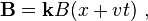
Lorentz force law version
The Maxwell-Faraday equation says the moving observer sees an electric field Ey in the y-direction given by:


![\mathcal{E} = -\ell [ E_y (x_C+w/2,\ t) - E_y(x_C-w/2,\ t)]](http://upload.wikimedia.org/math/3/b/9/3b950e184ab5d52e2b6aae534a14559a.png)
![= v\ell [ B(x_C+w/2+v t) - B(x_C-w/2+vt)] \ ,](http://upload.wikimedia.org/math/3/c/a/3cacfe084d17fddf872aba14304b720e.png)
Faraday's law of induction
Using Faraday's law of induction, the observer moving with xC sees a changing magnetic flux, but the loop does not appear to move: the center of the loop xC is fixed because the moving observer is moving with the loop. The flux is then:


![=v\ell \ [ B(x_C+w/2+vt) - B(x_C-w/2+vt)] \ ,](http://upload.wikimedia.org/math/8/0/3/803906ede26061c543f9a171c6d242e7.png)
The stationary observer thought the EMF was a motional EMF, while the moving observer thought it was an induced EMF.[21]
Electrical generator

Main article: electrical generator
The EMF generated by Faraday's law of induction due to relative movement of a circuit and a magnetic field is the phenomenon underlying electrical generators. When a permanent magnet is moved relative to a conductor, or vice versa, an electromotive force is created. If the wire is connected through an electrical load, current will flow, and thus electrical energy is generated, converting the mechanical energy of motion to electrical energy. For example, the drum generator is based upon Figure 4. A different implementation of this idea is the Faraday's disc, shown in simplified form in Figure 8. Note that either the analysis of Figure 5, or direct application of the Lorentz force law, shows that a solid conducting disc works the same way.In the Faraday's disc example, the disc is rotated in a uniform magnetic field perpendicular to the disc, causing a current to flow in the radial arm due to the Lorentz force. It is interesting to understand how it arises that mechanical work is necessary to drive this current. When the generated current flows through the conducting rim, a magnetic field is generated by this current through Ampere's circuital law (labeled "induced B" in Figure 8). The rim thus becomes an electromagnet that resists rotation of the disc (an example of Lenz's law). On the far side of the figure, the return current flows from the rotating arm through the far side of the rim to the bottom brush. The B-field induced by this return current opposes the applied B-field, tending to decrease the flux through that side of the circuit, opposing the increase in flux due to rotation. On the near side of the figure, the return current flows from the rotating arm through the near side of the rim to the bottom brush. The induced B-field increases the flux on this side of the circuit, opposing the decrease in flux due to rotation. Thus, both sides of the circuit generate an emf opposing the rotation. The energy required to keep the disc moving, despite this reactive force, is exactly equal to the electrical energy generated (plus energy wasted due to friction, Joule heating, and other inefficiencies). This behavior is common to all generators converting mechanical energy to electrical energy.
Although Faraday's law always describes the working of electrical generators, the detailed mechanism can differ in different cases. When the magnet is rotated around a stationary conductor, the changing magnetic field creates an electric field, as described by the Maxwell-Faraday equation, and that electric field pushes the charges through the wire. This case is called an induced EMF. On the other hand, when the magnet is stationary and the conductor is rotated, the moving charges experience a magnetic force (as described by the Lorentz force law), and this magnetic force pushes the charges through the wire. This case is called motional EMF. (For more information on motional EMF, induced EMF, Faraday's law, and the Lorentz force, see above example, and see Griffiths.)[22]
Electrical motor
Main article: electrical motor
An electrical generator can be run "backwards" to become a motor. For example, with the Faraday disc, suppose a DC current is driven through the conducting radial arm by a voltage. Then by the Lorentz force law, this traveling charge experiences a force in the magnetic field B that will turn the disc in a direction given by Fleming's left hand rule. In the absence of irreversible effects, like friction or Joule heating, the disc turns at the rate necessary to make d ΦB / dt equal to the voltage driving the current.Electrical transformer
Main article: transformer
The EMF predicted by Faraday's law is also responsible for electrical transformers. When the electric current in a loop of wire changes, the changing current creates a changing magnetic field. A second wire in reach of this magnetic field will experience this change in magnetic field as a change in its coupled magnetic flux, a d ΦB / d t. Therefore, an electromotive force is set up in the second loop called the induced EMF or transformer EMF. If the two ends of this loop are connected through an electrical load, current will flow.Magnetic flow meter
Main article: magnetic flow meter
Faraday's law is used for measuring the flow of electrically conductive liquids and slurries. Such instruments are called magnetic flow meters. The induced voltage ℇ generated in the magnetic field B due to a conductive liquid moving at velocity v is thus given by: ,
,
Parasitic induction and waste heating
All metal objects moving in relation to a static magnetic field will experience inductive power flow, as do all stationary metal objects in relation to a moving magnetic field. These power flows are occasionally undesirable, resulting in flowing electric current at very low voltage and heating of the metal.There are a number of methods employed to control these undesirable inductive effects.
- Electromagnets in electric motors, generators, and transformers do not use solid metal, but instead use thin sheets of metal plate, called laminations. These thin plates reduce the parasitic eddy currents, as described below.
- Inductive coils in electronics typically use magnetic cores to minimize parasitic current flow. They are a mixture of metal powder plus a resin binder that can hold any shape. The binder prevents parasitic current flow through the powdered metal.
Electromagnet laminations


Parasitic induction within inductors

This is one reason high voltage devices tend to be more efficient than low voltage devices. High voltage devices use many turns of small-gauge wire in motors, generators, and transformers. These many small turns of inductor wire in the electromagnet break up the eddy flows that can form within the large, thick inductors of low voltage, high current devices.
No comments:
Post a Comment